
TL;DR
Senators and Representatives are staying in office longer. I’m using R and the data from The United States Github Repo to take a look at this.
It is not the US Gov’t’s repo, it is a collaboration between folks with the Sunlight Foundation, GovTrack.us, the New York Times, the Electronic Frontier Foundation, and the Internet. Take a look at their website.
The Congress
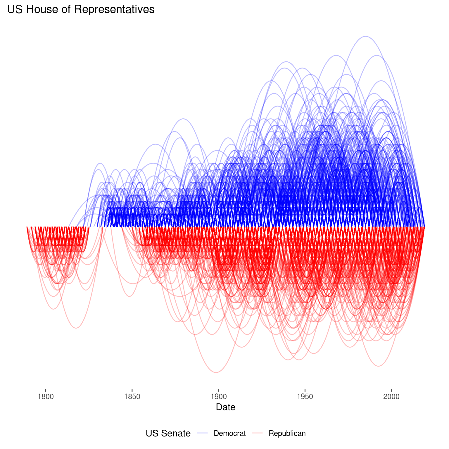

The above two images show Democrat and Republican legislators in both the US House and US Senate, for all legislators that are not currently serving (so @AOC and @DanCrenshawTX are not represented). The data begins with Bassett on 1789-03-04 and ends with Marino on 2019-01-23.
Party Time
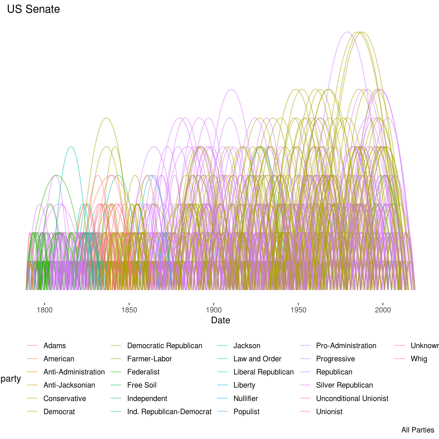
This image shows all the parties, for completeness. And while historically the “Nullifiers” certainly existed, they really haven’t had much to do since 1833-03-03, which is when Barnwell ended the final Nullifier term.
Durations
Back to this image of the Senate:
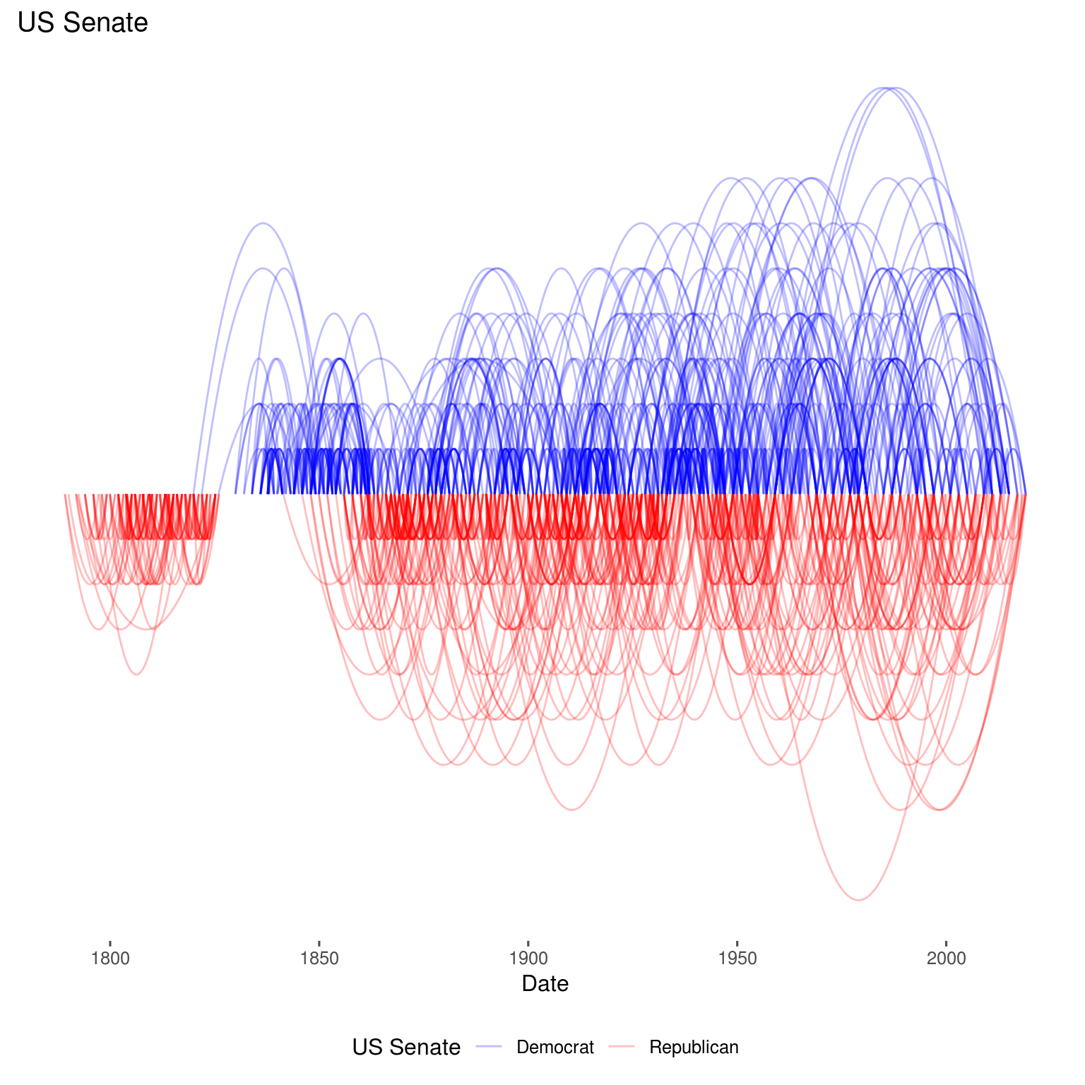
Each arc represents the one Senator’s contiguous service to the United States. Imagine a timeline drawn through the middle of the arcs (horizonatally) and the left point of each arc is where on the timeline that the service began. Similarly, the right hand side of the arc shows where the service ended. The distance between these two points is the duration of the service. The height of the arc is proportional to the duration as well, which probably violates multiple “rules of good data visualization” such as “never map the same value to more than one aesthetic”.
BUT…
The envelope of the arcs widens to the right (as time progresses), revealing that the legislators are serving longer. The arcs also form strata as well, which directly correspond to the number of terms served by each legislator.
We can see the duration increase here:
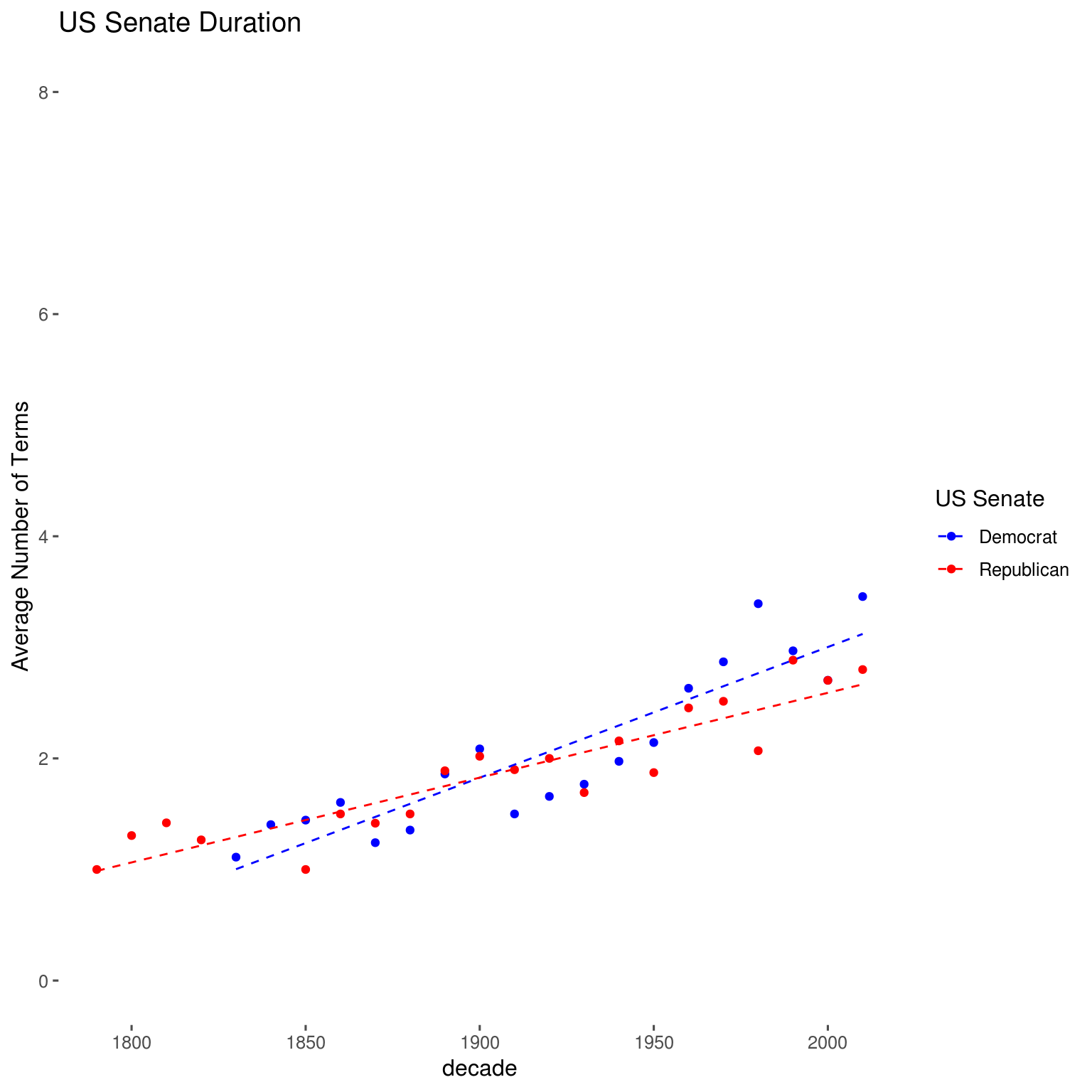
Over time, the average number of terms served has increased from 1 to between two and three, with Democrats tending to serve longer in recent years. I’m not much of a historian, but my understanding is that the orginal intent of the US Congress was as a “part time job”. Legislators would come, legislate, and return back to their full-time jobs (the Constitution states that Congress must meet at least once a year, but is mute on session-length). The advantages of seniority in the Legistlature have pretty much displaced the part-time nature - the more senior the Legistlator, the more effective in representing constituents.
Gender
We can take a look at gender in the legislatures as well. It might be easiest to only look at the “outlier” gender, which we can find easy enough:
| gender | type | n |
|---|---|---|
| F | rep | 208 |
| F | sen | 26 |
| M | rep | 10503 |
| M | sen | 1237 |
Female is the minority gender in both the House and the Senate; filtering for only “Female”, the “arc chart” for the House looks like:
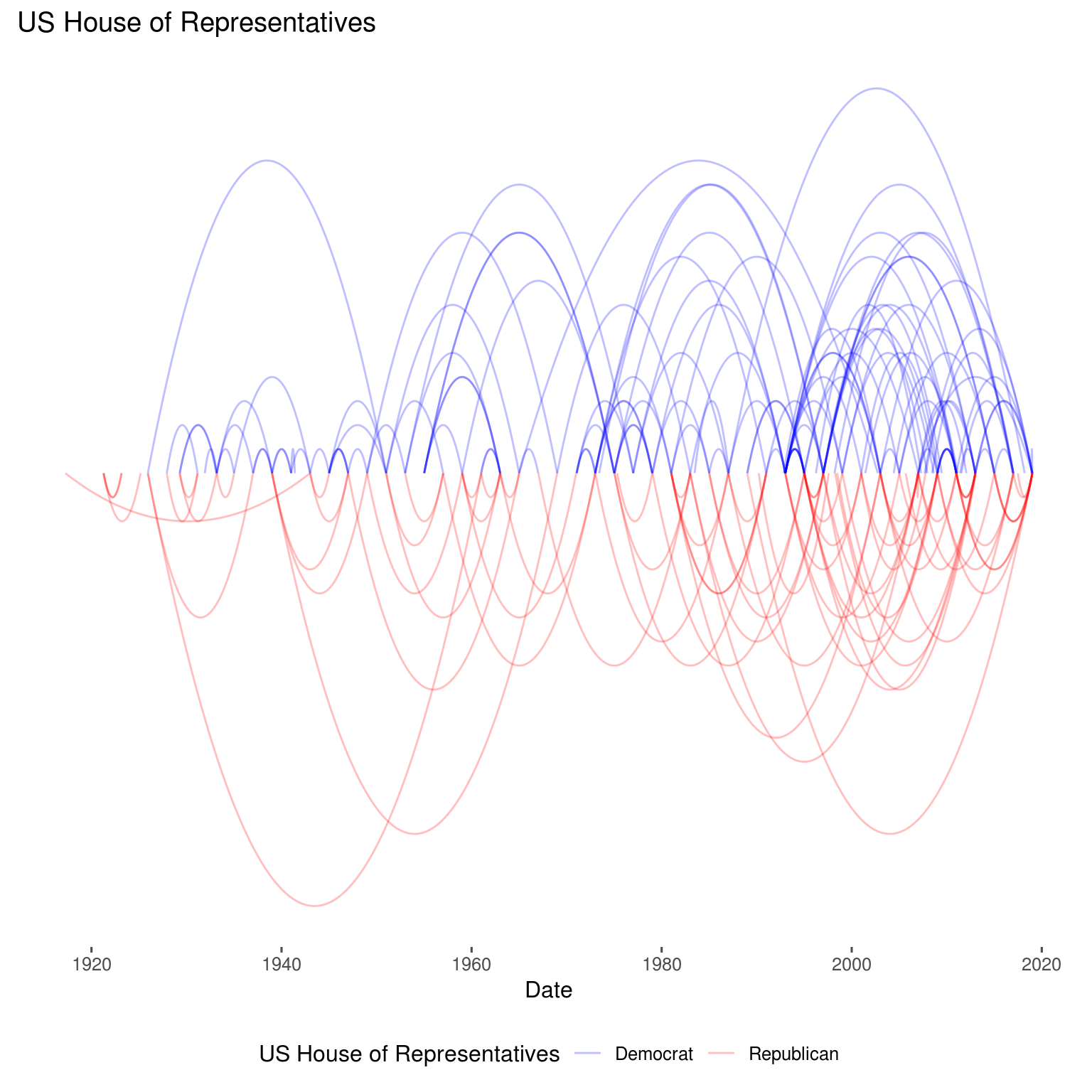
That very first arc is Jeannette Rankin, from the Great State of Montana. Interestingly, the data starts just before 1920 (Rankin was first elected on 1917-04-02). What happened in 1920? Oh yeah, the Nineteenth Amendment. Turns out that once you give a segment of the population the right to vote, that segment becomes represented (props to Montana for jumping the gun by a couple of years).
Recall that none of this data has currently serving legislators (but that data is in another data set - legislators_current.yaml).
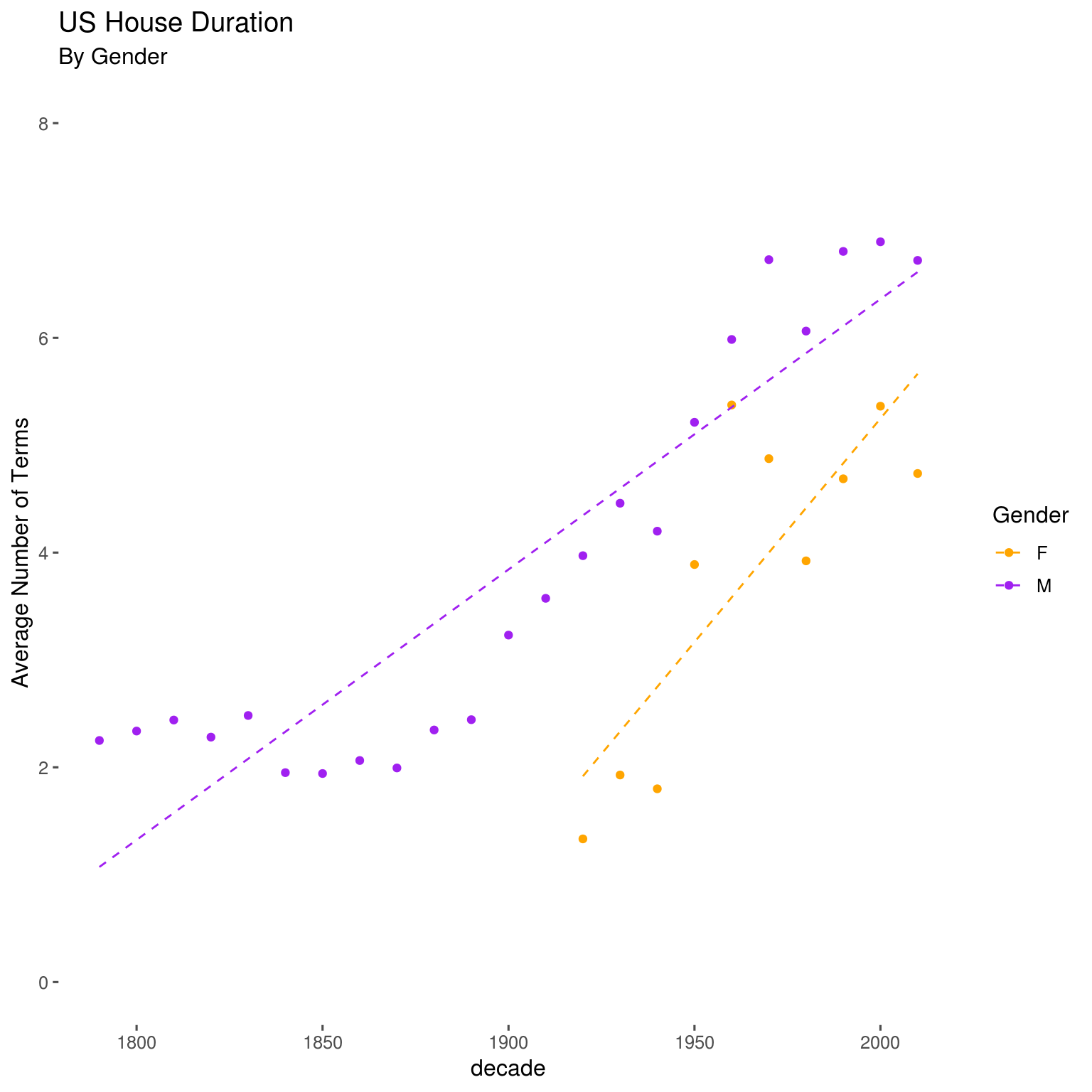
Women Representatives got a late start, but seem to be catching up.
Technical Details
This post was written in Rmarkdown and published via the Hugo static site generator. The source of this data-driven-document is up on github, but some of the more interesting technical details are below.
YAML
The source data is a YAML file, and the R yaml is used to read it.
load_file <- function(urlpath){
  yaml.load_file(url(urlpath))
}

fs <- cache_filesystem("./cache")

m_load_file <- memoise(load_file, cache = fs)

ledge <- m_load_file("https://github.com/unitedstates/congress-legislators/blob/master/legislators-historical.yaml?raw=true")
I used the memoise package to wrap the network access; this helped when authoring by creating a local copy of the ledge list. Memoise is pretty cool.
Beziers
The “arc plots” make heavy use of geom_bezier from ggforce. I used ggforce over ggalt due to package dependencies: ggalt wants to install proj4 which was a little too heavy for me.
One tricky part: after converting the yaml to a tibble, I had data that looked like
ledge_df %>% select(id, start, end) %>% top_n(3, id) %>% knitr::kable()| id | start | end |
|---|---|---|
| 412734 | 2017-02-09 | 2018-01-03 |
| 412737 | 2017-06-26 | 2019-01-03 |
| 412752 | 2018-11-29 | 2019-01-03 |
start and end map nicely to the x-axis, but I needed a height as well, so I used the numTerms. geom_bezier needs three control points for the Bezier curve: two on the x-axis and one off of the x-axis; I put the off-x-axis point at the midway between start and end with a y-corrdinate equaling numTerms. My tibble then looked like:
ledge_df %>% select(id, start, end, mid, numTerms) %>% top_n(3, id) %>% knitr::kable()| id | start | end | mid | numTerms |
|---|---|---|---|---|
| 412734 | 2017-02-09 | 2018-01-03 | 2017-07-23 | -1 |
| 412737 | 2017-06-26 | 2019-01-03 | 2018-03-31 | -1 |
| 412752 | 2018-11-29 | 2019-01-03 | 2018-12-17 | 1 |
But geom_bezier isn’t quite happy with this. It needs each point as a separate row, all grouped by some variable to define the curve. This is a tidyr problem, specifically tidyr::gather. I also needed to create a curve-id by pasteing the existing id with the start of the streak (this handled a legistlator (defined by the ‘id’ who had more than one streak)).
It all looked like:
ledge_df_long <- ledge_df %>%
  gather(key="event", value = "date", start, mid, end) %>%
  arrange(id) %>%
  mutate(spline_ctl_pt = numTerms) %>%
  mutate(spline_ctl_pt = if_else(event == "start", 0L, spline_ctl_pt)) %>%
  mutate(spline_ctl_pt = if_else(event == "end", 0L, spline_ctl_pt))
After which, I had a long tibble that looks like:
ledge_df_long %>% select(streak_id, event, date, spline_ctl_pt) %>% top_n(3, streak_id) %>% knitr::kable()| streak_id | event | date | spline_ctl_pt |
|---|---|---|---|
| 4127522018-11-29 | start | 2018-11-29 | 0 |
| 4127522018-11-29 | mid | 2018-12-17 | 1 |
| 4127522018-11-29 | end | 2019-01-03 | 0 |
which was used in geom_bezier:
ledge_df_long %>%
  filter(party %in% c("Democrat", "Republican")) %>%
  filter(type == "sen") %>%
  ggplot(aes(x=date, y=spline_ctl_pt, group=streak_id)) +
  geom_bezier(aes(color = party), alpha = 0.25) +
  scale_color_manual("US Senate", values=c("blue", "red")) +
  theme_few() + theme(legend.position = "bottom",
                      axis.text.y = element_blank(),
                      axis.title.y = element_blank(),
                      axis.ticks.y = element_blank(),
                      panel.border = element_blank()) +
  labs(
    title = "US Senate",
    x = "Date"
  )